Bisect Plot Examples

Introduction

This notebook explains the use case of the prepare_datasets, and plot_bisect functions from the Plaid library. The function is used to generate bisect plots for different scenarios using file paths and PLAID objects.

# Importing Required Libraries
from pathlib import Path
import os

from plaid import Dataset
from plaid.post.bisect import plot_bisect, prepare_datasets
from plaid import ProblemDefinition

# Setting up Directories
try:
    dataset_directory = Path(__file__).parent.parent.parent / "tests" / "post"
except NameError:
    dataset_directory = Path("..") / ".." / ".." / ".." / "tests" / "post"

Prepare Datasets for comparision

Assuming you have reference and predicted datasets, and a problem definition, The prepare_datasets function is used to obtain output scalars for subsequent analysis.

# Load PLAID datasets and problem metadata objects
ref_ds = Dataset(dataset_directory / "dataset_ref")
pred_ds = Dataset(dataset_directory / "dataset_near_pred")
problem = ProblemDefinition(dataset_directory / "problem_definition")

# Get output scalars from reference and prediction dataset
ref_out_scalars, pred_out_scalars, out_scalars_names = prepare_datasets(
    ref_ds, pred_ds, problem, verbose=True
)

print(f"{out_scalars_names = }\n")

  0%|          | 0/30 [00:00<?, ?it/s]

100%|██████████| 30/30 [00:00<00:00, 320992.65it/s]

out_scalars_names = ['scalar_2']

# Get output scalar
key = out_scalars_names[0]

print(f"KEY '{key}':\n")
print(f"ID{' ' * 5}--REF_out_scalars--{' ' * 7}--PRED_out_scalars--")

# Print output scalar values for both datasets
index = 0
for item1, item2 in zip(ref_out_scalars[key], pred_out_scalars[key]):
    print(
        f"{str(index).ljust(2)}  |  {str(item1).ljust(20)}  |   {str(item2).ljust(20)}"
    )
    index += 1

KEY 'scalar_2':

ID     --REF_out_scalars--       --PRED_out_scalars--
0   |  1.2169346066887108    |   1.3169346066887109  
1   |  0.515145770522403     |   0.555145770522403   
2   |  -3.9642788741978805   |   -3.8642788741978804 
3   |  -1.1124922797133046   |   -1.3124922797133045 
4   |  -1.4265630170876404   |   -1.1265630170876404 
5   |  0.6803811300084939    |   0.6703811300084939  
6   |  -0.8030708857345106   |   -0.8130708857345106 
7   |  -0.8807308582456169   |   -0.8807308582456169 
8   |  -0.4056076599154201   |   -0.4056076599154201 
9   |  -0.957992110650768    |   -0.957992110650768  
10  |  -0.625817777628713    |   -0.625817777628713  
11  |  1.096843506332501     |   1.596843506332501   
12  |  -0.11847882336841341  |   -0.07847882336841341
13  |  -1.2157807923268915   |   -1.1157807923268914 
14  |  1.1496798915782924    |   0.7496798915782924  
15  |  -0.7559990261696361   |   -0.7859990261696361 
16  |  1.4240494564951343    |   1.7240494564951343  
17  |  -1.5766265405726547   |   -1.8766265405726548 
18  |  0.3553127427434973    |   0.3553127427434973  
19  |  0.30428626244214857   |   0.30428626244214857 
20  |  1.1401354236737495    |   1.1401354236737495  
21  |  0.630121156724546     |   0.630121156724546   
22  |  0.017149879978562026  |   0.016149879978562025
23  |  0.2851246751356392    |   0.2751246751356392  
24  |  -0.1766974544661193   |   -0.1716974544661193 
25  |  0.7868416541432641    |   0.7818416541432641  
26  |  0.4158359150220023    |   0.4198359150220023  
27  |  0.5327780239393215    |   0.5367780239393215  
28  |  -0.05411433228195642  |   -0.05416433228195642
29  |  -0.6613558643195047   |   -0.6608558643195047 

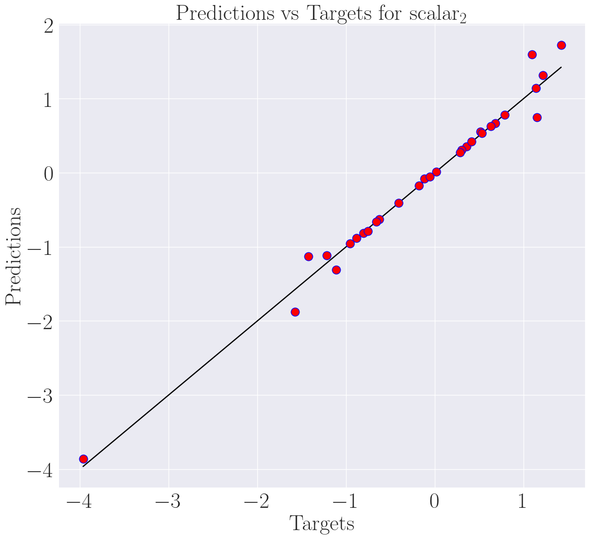
Plotting with File Paths

Here, we load the datasets and problem metadata from file paths and use the plot_bisect function to generate a bisect plot for a specific scalar, in this case, “scalar_2.”

print("=== Plot with file paths ===")

# Load PLAID datasets and problem metadata from files
ref_path = dataset_directory / "dataset_ref"
pred_path = dataset_directory / "dataset_pred"
problem_path = dataset_directory / "problem_definition"

# Using file paths to generate bisect plot on scalar_2
plot_bisect(ref_path, pred_path, problem_path, "scalar_2", "differ_bisect_plot")

=== Plot with file paths ===

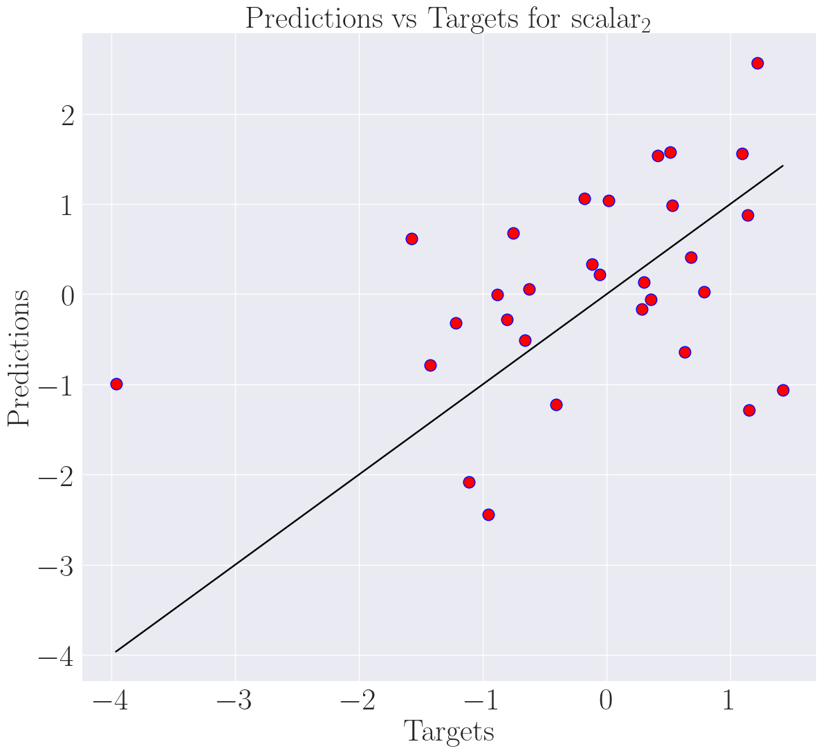
Plotting with PLAID

In this section, we demonstrate how to use PLAID objects directly to generate a bisect plot. This can be advantageous when working with PLAID datasets in memory.

print("=== Plot with PLAID objects ===")

# Load PLAID datasets and problem metadata objects
ref_path = Dataset(dataset_directory / "dataset_ref")
pred_path = Dataset(dataset_directory / "dataset_pred")
problem_path = ProblemDefinition(dataset_directory / "problem_definition")

# Using PLAID objects to generate bisect plot on scalar_2
plot_bisect(ref_path, pred_path, problem_path, "scalar_2", "equal_bisect_plot")

=== Plot with PLAID objects ===

Mixing with Scalar Index and Verbose

In this final section, we showcase a mix of file paths and PLAID objects, incorporating a scalar index and enabling the verbose option when generating a bisect plot. This can provide more detailed information during the plotting process.

print("=== Mix with scalar index and verbose ===")

# Mix
ref_path = dataset_directory / "dataset_ref"
pred_path = dataset_directory / "dataset_near_pred"
problem_path = ProblemDefinition(dataset_directory / "problem_definition")

# Using scalar index and verbose option to generate bisect plot
scalar_index = 0
plot_bisect(
    ref_path,
    pred_path,
    problem_path,
    scalar_index,
    "converge_bisect_plot",
    verbose=True,
)

os.remove("converge_bisect_plot.png")
os.remove("differ_bisect_plot.png")
os.remove("equal_bisect_plot.png")

=== Mix with scalar index and verbose ===
Data preprocessing...

  0%|          | 0/30 [00:00<?, ?it/s]

100%|██████████| 30/30 [00:00<00:00, 315361.20it/s]

Bisect graph construction...
Bisect graph saving...

...Bisect plot done