Bisect Plot Examples

Introduction

This notebook explains the use case of the prepare_datasets, and plot_bisect functions from the Plaid library. The function is used to generate bisect plots for different scenarios using file paths and PLAID objects.

# Importing Required Libraries
from pathlib import Path
import os

from plaid import Dataset
from plaid.post.bisect import plot_bisect, prepare_datasets
from plaid import ProblemDefinition

# Setting up Directories
try:
    dataset_directory = Path(__file__).parent.parent.parent / "tests" / "post"
except NameError:
    dataset_directory = Path("..") / ".." / ".." / ".." / "tests" / "post"

Prepare Datasets for comparision

Assuming you have reference and predicted datasets, and a problem definition, The prepare_datasets function is used to obtain output scalars for subsequent analysis.

# Load PLAID datasets and problem metadata objects
ref_ds = Dataset(dataset_directory / "dataset_ref")
pred_ds = Dataset(dataset_directory / "dataset_near_pred")
problem = ProblemDefinition(dataset_directory / "problem_definition")

# Get output scalars from reference and prediction dataset
ref_out_scalars, pred_out_scalars, out_scalars_names = prepare_datasets(
    ref_ds, pred_ds, problem, verbose=True
)

print(f"{out_scalars_names = }\n")

/tmp/ipykernel_3425/4066271457.py:7: DeprecationWarning: use `get_out_features_identifiers` instead [since v0.1.8] (will be removed in v0.2.0)
  ref_out_scalars, pred_out_scalars, out_scalars_names = prepare_datasets(

  0%|          | 0/30 [00:00<?, ?it/s]

100%|██████████| 30/30 [00:00<00:00, 36588.87it/s]

out_scalars_names = ['feature_2']

# Get output scalar
key = out_scalars_names[0]

print(f"KEY '{key}':\n")
print(f"ID{' ' * 5}--REF_out_scalars--{' ' * 7}--PRED_out_scalars--")

# Print output scalar values for both datasets
index = 0
for item1, item2 in zip(ref_out_scalars[key], pred_out_scalars[key]):
    print(
        f"{str(index).ljust(2)}  |  {str(item1).ljust(20)}  |   {str(item2).ljust(20)}"
    )
    index += 1

KEY 'feature_2':

ID     --REF_out_scalars--       --PRED_out_scalars--
0   |  0.6026743950988548    |   0.6026804218428058  
1   |  0.4010294552789103    |   0.40103346557346314 
2   |  0.4594691101022568    |   0.4594737047933578  
3   |  0.1734062211920243    |   0.17340795525423625 
4   |  0.21668654508983876   |   0.21668871195528966 
5   |  0.2181819183396143    |   0.21818410015879772 
6   |  0.5203262339832092    |   0.5203314372455491  
7   |  0.6797440087453753    |   0.6797508061854628  
8   |  0.7589424187607021    |   0.7589500081848898  
9   |  0.6345020332023174    |   0.6345083782226494  
10  |  0.7550570027405668    |   0.7550645533105942  
11  |  0.11902182132257      |   0.11902301154078324 
12  |  0.2277144265635649    |   0.22771670370783054 
13  |  0.26104884230989456   |   0.26105145279831765 
14  |  0.7418202872333769    |   0.7418277054362493  
15  |  0.8670795819513495    |   0.867088252747169   
16  |  0.9819893923184365    |   0.9819992122123598  
17  |  0.14881640806200802   |   0.14881789622608865 
18  |  0.10477886888726429   |   0.10477991667595317 
19  |  0.8075981575733645    |   0.8076062335549403  
20  |  0.11251682284184616   |   0.11251794801007459 
21  |  0.6874297933397363    |   0.6874366676376698  
22  |  0.6063536260025336    |   0.6063596895387937  
23  |  0.6013786933270137    |   0.601384707113947   
24  |  0.30270251139317916   |   0.3027055384182931  
25  |  0.49927569741356614   |   0.49928069017054033 
26  |  0.43825290644848336   |   0.4382572889775479  
27  |  0.46219564786354983   |   0.4622002698200285  
28  |  0.9643573718446001    |   0.9643670154183186  
29  |  0.09651135295899105   |   0.09651231807252064 

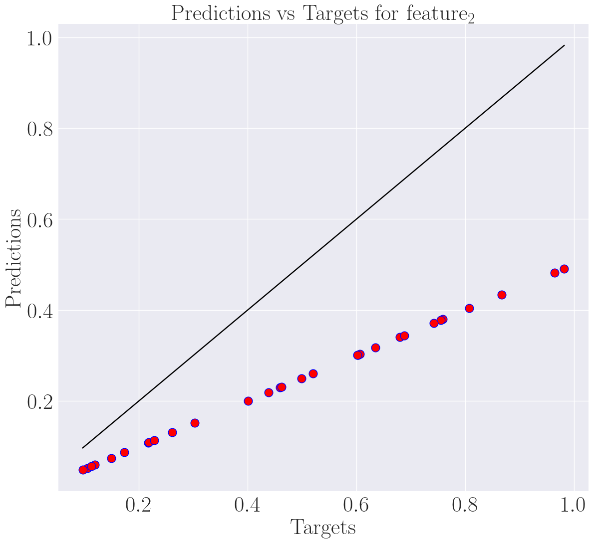
Plotting with File Paths

Here, we load the datasets and problem metadata from file paths and use the plot_bisect function to generate a bisect plot for a specific scalar, in this case, “scalar_2.”

print("=== Plot with file paths ===")

# Load PLAID datasets and problem metadata from files
ref_path = dataset_directory / "dataset_ref"
pred_path = dataset_directory / "dataset_pred"
problem_path = dataset_directory / "problem_definition"

# Using file paths to generate bisect plot on feature_2
plot_bisect(ref_path, pred_path, problem_path, "feature_2", "differ_bisect_plot")

=== Plot with file paths ===

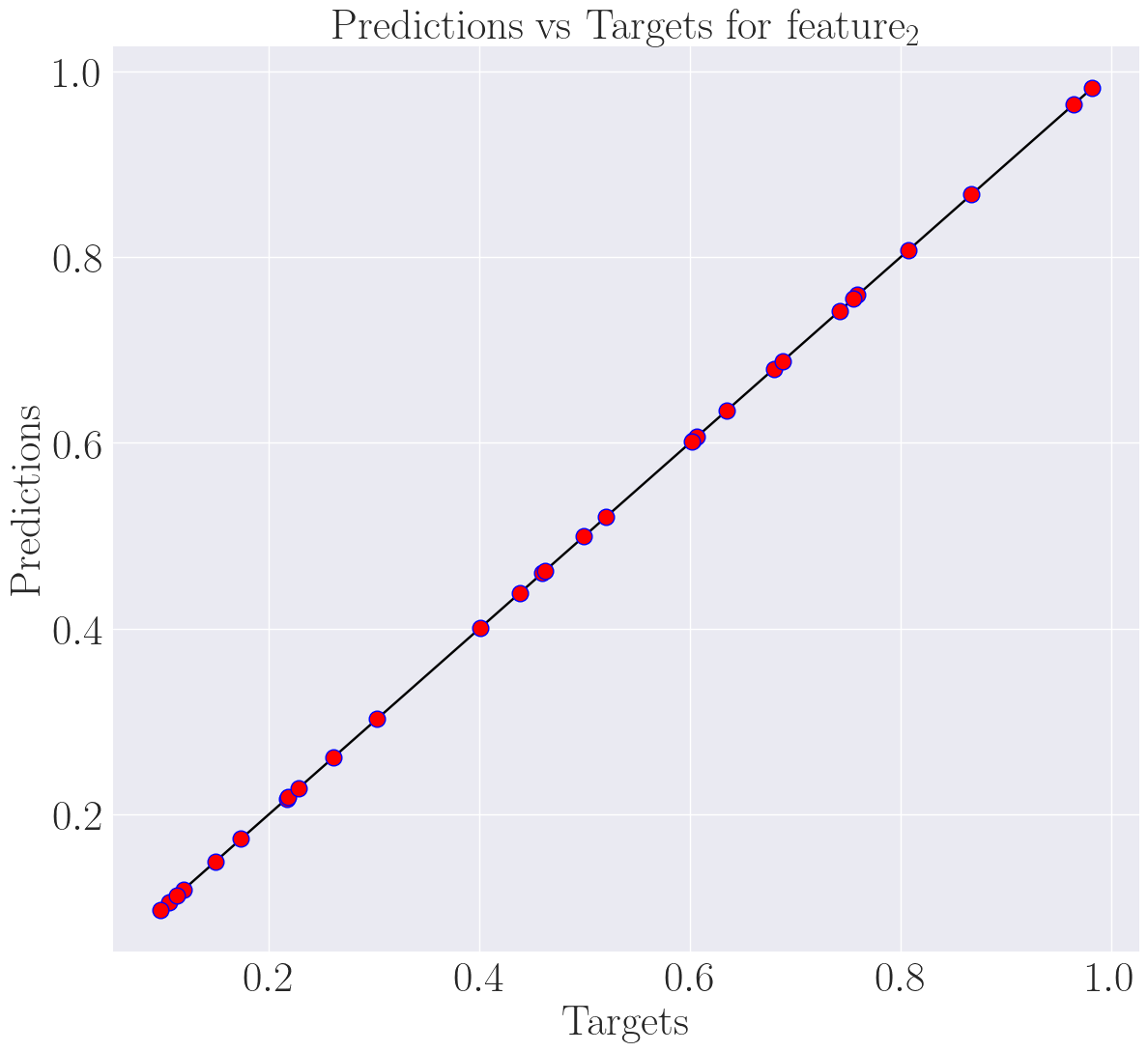
Plotting with PLAID

In this section, we demonstrate how to use PLAID objects directly to generate a bisect plot. This can be advantageous when working with PLAID datasets in memory.

print("=== Plot with PLAID objects ===")

# Load PLAID datasets and problem metadata objects
ref_path = Dataset(dataset_directory / "dataset_ref")
pred_path = Dataset(dataset_directory / "dataset_pred")
problem_path = ProblemDefinition(dataset_directory / "problem_definition")

# Using PLAID objects to generate bisect plot on feature_2
plot_bisect(ref_path, pred_path, problem_path, "feature_2", "equal_bisect_plot")

=== Plot with PLAID objects ===

Mixing with Scalar Index and Verbose

In this final section, we showcase a mix of file paths and PLAID objects, incorporating a scalar index and enabling the verbose option when generating a bisect plot. This can provide more detailed information during the plotting process.

print("=== Mix with scalar index and verbose ===")

# Mix
ref_path = dataset_directory / "dataset_ref"
pred_path = dataset_directory / "dataset_near_pred"
problem_path = ProblemDefinition(dataset_directory / "problem_definition")

# Using scalar index and verbose option to generate bisect plot
scalar_index = 0
plot_bisect(
    ref_path,
    pred_path,
    problem_path,
    scalar_index,
    "converge_bisect_plot",
    verbose=True,
)

os.remove("converge_bisect_plot.png")
os.remove("differ_bisect_plot.png")
os.remove("equal_bisect_plot.png")

=== Mix with scalar index and verbose ===
Data preprocessing...

  0%|          | 0/30 [00:00<?, ?it/s]

100%|██████████| 30/30 [00:00<00:00, 22786.87it/s]

Bisect graph construction...
Bisect graph saving...

...Bisect plot done